
Predicting house prices in Ames, IA
This is a rerun of a project I did while in General Assembly’s Data Science Immersive program. While editing the notebook for posting here, I ended up completely redoing it, having learned more since its first version.
Ames dataset is notoriously unruly, with 80 features and a good chunk of missing values, so the focus of this work is data cleaning and feature selection. As such, the features contrasted here are the ones determined by:
- My common sense, 24 of those conventionally thought of as influencing house prices
- Pearson correlation coefficient (.corr method), top 24 of those - to match ones selected by me
- Principle Component Analysis, the most popular dimensionality reduction algorithm that transforms original variables onto the new axes
- Recursive Feature Elimination, method that fits successive versions of a model and drops the least informative ones
- Lasso regularization, a regularized version of Linear Regression that eliminates the weights of the least important features.
As the notebook below shows, this competition against statistical algorithms was lost by the human, i.e. feature set number 1 did worse in predicting house prices than the other features, PCA predicting the best.
The modelling, hyperparameter tuning and evaluation (cross-val score is used for a quick look at the model) is bare bones, not to take away the attention from the feature selection.
Lastly, I’ve put all the processing steps in a pipeline, taking up one code box in the very end. The results in the pipeline are different, most likely due to its sweeping method of dealing with the missing values.
import pandas as pd
import numpy as np
train = pd.read_csv('train.csv')
test = pd.read_csv('test.csv')
MISSING VALUES
print("Shape of Original DataFrame: {}".format(train.shape))
Shape of Original DataFrame: (1460, 81)
# dropping the features with around half of value,
# since we cannot legitimately infer what the missing values might stand for and therefore impute them
train = train.drop(['PoolQC', 'MiscFeature', 'Alley', 'Fence', 'FireplaceQu'], axis=1)

# dropping features of Garage and BSMT group, since they are interchangeable
train = train.drop(['GarageCond', 'GarageFinish', 'GarageQual', 'GarageType', 'GarageYrBlt'], axis=1)
train = train.drop(['BsmtCond', 'BsmtExposure', 'BsmtFinType1', 'BsmtFinType2', 'BsmtQual'], axis=1)

# dropping the relatively/sujectively unimportant
train = train.drop(['MasVnrArea', 'MasVnrType'], axis=1)
train = train.drop(train.loc[train['Electrical'].isnull()].index)

# LotFrontage: NA most likely means no lot frontage
train.loc[:, "LotFrontage"] = train.loc[:, "LotFrontage"].fillna(0)
print("Shape of DataFrame After Dropping All Rows with Missing Values: {}".format(train.shape))
Shape of DataFrame After Dropping All Rows with Missing Values: (1459, 64)
FEATURES
But first, the predictor:
import matplotlib.pyplot as plt
%matplotlib inline
plt.hist(train.SalePrice, color='gold')
plt.show()
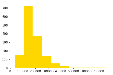
The distribution is positively skewed (a longer tail on the right), so we need to log-transform the target variable to improve the linearity of the data.
y = np.log(train['SalePrice'].ravel()).copy()
Now back to features.
from sklearn.preprocessing import StandardScaler
from sklearn.linear_model import LinearRegression, Lasso
from sklearn.model_selection import cross_val_score, cross_val_predict
from sklearn.decomposition import PCA
from sklearn.feature_selection import RFE
# CONVENTIONAL
quality = train[['OverallQual', 'KitchenQual', 'ExterQual', 'LowQualFinSF', 'HeatingQC']]
footage = train[['TotalBsmtSF', 'GrLivArea', 'GarageArea', 'PoolArea', 'LotArea']]
neighborhood = train[['MSSubClass', 'LandContour', 'Neighborhood', 'BldgType']]
age = train[['YearBuilt', 'YearRemodAdd', 'YrSold']]
property_attr = train[['Foundation', 'Exterior1st', 'Utilities']]
rooms = train[['FullBath', 'BedroomAbvGr', 'Fireplaces', 'GarageCars']]
conventional = pd.get_dummies(pd.concat([quality, footage, neighborhood, age, property_attr, rooms], axis=1))

# ALL
allfeatures = pd.get_dummies(train[[col for col in train.columns if col !='SalePrice']].copy(), drop_first=True)

# CORRELATED
top24 = ss.fit_transform(pd.get_dummies(train[['OverallQual', 'GrLivArea', 'TotalBsmtSF', 'GarageCars', 'GarageArea',
                    '1stFlrSF', 'FullBath', 'TotRmsAbvGrd', 'YearBuilt', 'YearRemodAdd',
                    'Fireplaces', 'BsmtFinSF1', 'LotFrontage', 'SaleCondition', 'WoodDeckSF',
                    '2ndFlrSF', 'OpenPorchSF', 'HalfBath', 'LotArea', 'BsmtFullBath',
                    'BsmtUnfSF', 'BedroomAbvGr', 'ScreenPorch', 'PoolArea']]))
ss = StandardScaler()
allfeatures_scaled = ss.fit_transform(allfeatures)
conventional_scaled = ss.fit_transform(conventional)
top24_scaled = ss.fit_transform(top24)
# PCA
pca = PCA(n_components=24)
pca_features = pca.fit_transform(allfeatures_scaled)

# RFE
rfe = RFE(lr, n_features_to_select=48)
rfe.fit(allfeatures_scaled, y)
rfe_features = allfeatures.iloc[:, rfe.support_]

# Lasso
from sklearn.feature_selection import SelectFromModel
lasso = Lasso()
lasso.fit(allfeatures, y)
lasso_features = SelectFromModel(lasso, prefit=True).transform(allfeatures_scaled)
print("%s variables of %s where removed"%(sum(lasso.coef_ == 0), len(lasso.coef_)),'\n')

# To see columns chosen by Lasso
for col, coef in zip(allfeatures.columns, lasso.coef_):
        if coef != 0.0:
            print('Use', col, coef)
182 variables of 194 where removed

Use Id -9.25448035226e-06
Use LotArea 1.57170015403e-06
Use YearBuilt 0.00251265135532
Use YearRemodAdd 0.00124464719792
Use BsmtFinSF1 4.75616875206e-05
Use TotalBsmtSF 0.000163445309797
Use 2ndFlrSF 2.24344702183e-05
Use GrLivArea 0.000310610759168
Use GarageArea 0.000386175392281
Use WoodDeckSF 0.000159391904829
Use ScreenPorch 0.00013472881683
Use MiscVal -5.63585179224e-08
SCORING
# Baseline model predicting the mean
from sklearn.metrics import r2_score
train['baseline'] = y.mean()
print('Score of predicting the mean:', r2_score(train['SalePrice'], train['baseline']))
Score of predicting the mean: -5.18642379411
# Just the Linear Regression model
lr = LinearRegression()
print('Score of LR using all features:', cross_val_score(lr, allfeatures_scaled, y, cv=5).mean())
print('Score of LR using conventional features:', cross_val_score(lr, conventional_scaled, y, cv=5).mean())
print('Score LR via .corr:', cross_val_score(lr, top24_scaled, y, cv=5).mean())
Score of LR using all features: -3.42869523964e+25
Score of LR using conventional features: -9.14521643608e+25
Score LR via .corr: 0.830148489466
print('Score via PCA:', cross_val_score(lr, pca_features, y, cv=5).mean())
Score via PCA: 0.822915445903
print('Score via Lasso:', cross_val_score(lr, lasso_features, y, cv=5).mean())
Score via Lasso: 0.768549011367
print('Score via RFE:', cross_val_score(lr, rfe_features, y, cv=5).mean())
Score via RFE: 0.787283940054
Same in a PIPELINE
from sklearn.preprocessing import Imputer
from sklearn.pipeline import Pipeline
X = allfeatures
imputing = ('imputing', Imputer(missing_values=0, strategy='mean', axis=0))
scaling = ('scaling', StandardScaler())
rfe = ('rfe', RFE(lr, n_features_to_select=24, step=5))
pca = ('pca', PCA(n_components=24))
lrp = ('lrp', LinearRegression())
lasso = ('lasso', Lasso())

lr_pipeline = Pipeline([imputing, scaling, lrp])
lr_pipeline.fit(conventional, y)

rfe_pipeline = Pipeline([imputing, scaling, rfe]) # Create the pipeline: pipeline
rfe_pipeline.fit(X, y) # Fit the pipeline to the train set

pca_pipeline = Pipeline([imputing, scaling, pca, lrp])
pca_pipeline.fit(X, y)

lasso_pipeline = Pipeline([imputing, scaling, lasso]) # Create the pipeline: pipeline
lasso_features = SelectFromModel(Lasso().fit(X, y), prefit=True).transform(X)

print('LR score, conv:', cross_val_score(lr_pipeline, conventional, y, cv=5).mean())
print('LR score, top24:', cross_val_score(lr_pipeline, top24, y, cv=5).mean())
print('PCA score:', cross_val_score(pca_pipeline, X, y, cv=5).mean())
print('RFE score:', cross_val_score(rfe_pipeline, X, y).mean())
print('Lasso score:', cross_val_score(lr, lasso_features, y, cv=5).mean())
LR score, conv: 0.812249293965
LR score, top24: 0.830349597185
PCA score: 0.802999116798
RFE score: 0.822382038559
Lasso score: 0.768549011367