Project: Model interpretability and imbalanced datasets in predicting Home Credit Default Risk.
This is an imbalanced class project with focus on interpreting the result of a simple classification model.
Imbalanced data / rare event
We’re going to predict mortgage default risk, with target class distribution severely skewed towards the non-defaults. Such imbalance is common in areas like fraud detection, medical diagnosis, manufacturing defects, and risk management and the problem of a rare event prediction and is a fascinating one to solve. Traditional statistical tools like probability are not very helpful here, as in those problems, it’s that 1% the model says nothing about that’s going to mess you up (tail risk). In order to obtain a fair balance in the number of instances for both the classes, a sampling technique is suggested, whereby we are re-balancing classes in the training data thus magnifying those unlikely events that’s hard to see.
Interpretability
Analysis is only as valuable as the explanation. This is something not discussed enough, including the bootcamp course I’ve graduated from and new online courses coming out from esteemed AI practitioners. What do we do with the model’s predictions once data has been fitted and performance evaluated? It’s been indeed a black box to me.
On the broader, society-level, we are increasingly dependent on intelligent machines, powered by the surge in the capabilities of black-box techniques, or algorithms whose inner workings cannot easily be explained, like deep learning. Yet the impact of algorithms on our experience of the world is growing.
For example, the system can detect that bipolar people tend to become overspenders, compulsive gamblers and target them at the onset of manic phase to buy tickets to Vegas. Platforms with the kind of power Facebook and Google have can decide to turn out supporters of one candidate over the other. Imagine what a state can do with the immense amount of data it has on its citizens. China is already using face detection technology to identify and arrest people.
As Zeynep Tufekci said in her great TED talk, with infrastructure designed to get people to click on ads, we’re building surveillance authoritarianism that can envelop us like a spider’s web and we may not even know we’re in it.
On a business-level, we want to not just predict probable outcomes, but also to answer the initial business question. In this notebook’s problem, the business decision is whether a borrower is going to repay their loan. A model can calculate probabilities of default, with which a lender can set a threshold, according to their risk tolerance, above which it’s willing to lend to the borrower, and below which it’ll flag the application for further review. (Interestingly, another type of risk banks might want to predict is a seemingly opposite risk of a customer prepaying the loan all at once, thus depriving the bank from their bread and butter, the interest payments.)
By law, credit companies have to be able to explain their denial-of-credit decisions. GDPR grants a right to an explanations why algorithm decided one way or another. Whether or not you have a law about it where you work, it might still make good sense for your business to have a simple way to explain the model’s decision. A model you can interpret and understand is one you can more easily improve, trust and reach decision insights with.
Logistic Regression
There is a central tension, however, between accuracy and interpretability: the most accurate models are necessarily the hardest to understand. Random forests, for example, have a high accuracy but are not very easy to interpret. Logistic regression, on the other hand, is a parametric linear model that has a lot of explanatory power. It also has the hyper-parameter “balanced” class_weight, which can be used as an algorithm-level technique. Being able to take its output and speak about it to someone who isn’t technical is a big plus. So if you don’t have years to spend understanding a result, give up some accuracy for simplicity of understanding.
Evaluation
The evaluation of classifier models is not as straightforward as regression models. It’s even more important to choose the evaluation metric correctly when assessing an imbalanced classification problem. As such if we simply predicted majority class in all cases, we would single-handedly achieve high accuracy (91.5% in our case). Instead we’ll be using the ROC AUC to evaluate the model.
The ROC shows the True Positive Rate versus the False Positive Rate as a function of the threshold according to which we classify an instance as positive. The True Positives are the important ones to get right, as the cost of False Negative is usually much larger than False Positive, yet ML algorithms penalize both at a similar weight. In credit risk, if we predict a loan will default yet it doesn’t, the maximum loss is the profit you’d have made by issuing that loan. On the other hand, if your model classifies a default loan as being safe, you will also lose the issued amount in addition to the foregone profit.
Interpretable machine learning tools help us decide and, more broadly, do better model validation. Practitioners agree that model validation should include answering questions such as: how does the model output relate to the value of each feature? Do these relations match human intuition and/or domain knowledge? What features weight the most for a specific observation?
Imports and basic transformations
import numpy as np
import pandas as pd
import seaborn as sns
import matplotlib.pyplot as plt
from sklearn.linear_model import LogisticRegression
from sklearn.preprocessing import Imputer, StandardScaler
from sklearn.model_selection import train_test_split, GridSearchCV
from sklearn.metrics import roc_curve, roc_auc_score, confusion_matrix, classification_report
%matplotlib inline
# upload some of the datasets available
app = pd.read_csv("application_train.csv")
previous_credits = pd.read_csv('bureau.csv')
# Groupby the client id and count the number of previous loans
previous_loan_counts = previous_credits.groupby('SK_ID_CURR', as_index=False)['SK_ID_BUREAU'].count().rename(columns = {'SK_ID_BUREAU': 'previous_loan_counts'})
df = app.merge(previous_loan_counts, on = 'SK_ID_CURR', how = 'left')
# Fill the missing values with 0
df['previous_loan_counts'] = df['previous_loan_counts'].fillna(0)
df.columns = map(str.lower, df.columns)
df.index.names = ['ID'] # 'SK_ID_CURR' is long and confusing
Target / the dependent variable
# bargraph of the distributions
sns.countplot(x='target', data=df)
plt.title('Class Frequency')
plt.xlabel('Class')
plt.ylabel('Frequency')
plt.show()
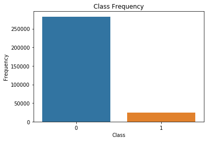
# distribution of target (skewed): If we were to always predict 0, we'd achieve an accuracy of 92%.
count_nondefault = len(df[df["target"]==0])
count_default = len(df[df["target"]==1])

percent_nondefault = (count_nondefault / (count_nondefault + count_default)) * 100
percent_default = (count_default / (count_nondefault + count_default)) * 100

percent_default, percent_nondefault
(8.072881945686495, 91.92711805431351)
Downsampling
Due to the inherent complex characteristics of an imbalanced dataset, learning from such data requires a special approach to transform data. One of such approaches are the sampling techniques which re-balances classes in the training data. The main idea of sampling classes is to either increasing the samples of the minority class or decreasing the samples of the majority class.
First, we separate observations from each class into different DataFrames. Next, we resample the majority class without replacement, setting the number of samples to match that of the minority class. Finally, we combine the down-sampled majority class DataFrame with the original minority class DataFrame.
The resampled technique did not improve the performance of the model, but I’ll leave the code here anyway.
from sklearn.utils import resample

# separate minority and majority classes
defaulted = df.loc[df.target==1, :]
nondefaulted = df.loc[df.target==0, :]

# Downsample majority class
df_majority_downsampled = resample(nondefaulted,
                                 replace=False,                # sample without replacement
                                 n_samples=len(defaulted)*2,   # to match minority class
                                 random_state=123)             # reproducible results
# Combine minority class with downsampled majority class
df_downsampled = pd.concat([df_majority_downsampled, defaulted])

# Display new class counts
df_downsampled.target.value_counts()
Finish EDA
# general overview of the numerical variables with the target classes
df.groupby('target').mean()
| sk_id_curr | cnt_children | amt_income_total | amt_credit | amt_annuity | amt_goods_price | region_population_relative | days_birth | days_employed | days_registration | ... | housetype_mode_terraced house | wallsmaterial_mode_Block | wallsmaterial_mode_Mixed | wallsmaterial_mode_Monolithic | wallsmaterial_mode_Others | wallsmaterial_mode_Panel | wallsmaterial_mode_Stone, brick | wallsmaterial_mode_Wooden | emergencystate_mode_No | emergencystate_mode_Yes | |
|---|---|---|---|---|---|---|---|---|---|---|---|---|---|---|---|---|---|---|---|---|---|
| target | |||||||||||||||||||||
| 0 | 278244.744536 | 0.412946 | 169077.722266 | 602648.282002 | 27163.623349 | 542736.795003 | 0.021021 | -16138.176397 | 65696.146123 | -5029.941065 | ... | 0.003923 | 0.030433 | 0.007510 | 0.005996 | 0.005271 | 0.218787 | 0.212303 | 0.017129 | 0.524695 | 0.007446 |
| 1 | 277449.167936 | 0.463807 | 165611.760906 | 557778.527674 | 26481.744290 | 488972.412554 | 0.019131 | -14884.828077 | 42394.675448 | -4487.127009 | ... | 0.004149 | 0.026183 | 0.006969 | 0.003384 | 0.005438 | 0.168862 | 0.193353 | 0.020947 | 0.447291 | 0.008983 |
2 rows × 246 columns
# check for anomalies
df.describe()
| sk_id_curr | target | cnt_children | amt_income_total | amt_credit | amt_annuity | amt_goods_price | region_population_relative | days_registration | days_id_publish | ... | wallsmaterial_mode_Panel | wallsmaterial_mode_Stone, brick | wallsmaterial_mode_Wooden | emergencystate_mode_No | emergencystate_mode_Yes | years_birth | years_employed | credit_bins | Credit_to_income | Goods_to_credit | |
|---|---|---|---|---|---|---|---|---|---|---|---|---|---|---|---|---|---|---|---|---|---|
| count | 300818.000000 | 300818.000000 | 300818.000000 | 300818.000000 | 3.008180e+05 | 300818.000000 | 3.008180e+05 | 300818.000000 | 300818.000000 | 300818.000000 | ... | 300818.000000 | 300818.000000 | 300818.000000 | 300818.000000 | 300818.000000 | 300818.000000 | 300818.000000 | 300818.000000 | 300818.000000 | 300818.000000 |
| mean | 278178.771722 | 0.081534 | 0.416870 | 164261.647540 | 5.716649e+05 | 26397.050699 | 5.126138e+05 | 0.020729 | -4993.488964 | -2993.503105 | ... | 0.213096 | 0.210057 | 0.017496 | 0.515471 | 0.007603 | 43.921554 | 6.505120 | 3.938415 | 1.123706 | 0.900233 |
| std | 102794.494538 | 0.273654 | 0.722093 | 84763.630041 | 3.549836e+05 | 13441.091525 | 3.238183e+05 | 0.013633 | 3525.082622 | 1508.545558 | ... | 0.409495 | 0.407350 | 0.131109 | 0.499761 | 0.086861 | 11.990418 | 5.780272 | 2.018892 | 0.124768 | 0.097172 |
| min | 100002.000000 | 0.000000 | 0.000000 | 25650.000000 | 4.500000e+04 | 1615.500000 | 4.050000e+04 | 0.000290 | -24672.000000 | -7197.000000 | ... | 0.000000 | 0.000000 | 0.000000 | 0.000000 | 0.000000 | 20.517808 | -0.000000 | 1.000000 | 0.150000 | 0.166667 |
| 25% | 189123.250000 | 0.000000 | 0.000000 | 112500.000000 | 2.700000e+05 | 16407.000000 | 2.385000e+05 | 0.010006 | -7489.000000 | -4297.000000 | ... | 0.000000 | 0.000000 | 0.000000 | 0.000000 | 0.000000 | 33.936986 | 2.547945 | 2.000000 | 1.000000 | 0.834725 |
| 50% | 278221.500000 | 0.000000 | 0.000000 | 144000.000000 | 5.084955e+05 | 24588.000000 | 4.500000e+05 | 0.018850 | -4510.000000 | -3253.000000 | ... | 0.000000 | 0.000000 | 0.000000 | 1.000000 | 0.000000 | 43.117808 | 6.063014 | 4.000000 | 1.118800 | 0.893815 |
| 75% | 367101.750000 | 0.000000 | 1.000000 | 202500.000000 | 7.915320e+05 | 33696.000000 | 6.750000e+05 | 0.028663 | -2019.000000 | -1720.000000 | ... | 0.000000 | 0.000000 | 0.000000 | 1.000000 | 0.000000 | 53.947945 | 7.520548 | 6.000000 | 1.198000 | 1.000000 |
| max | 456255.000000 | 1.000000 | 19.000000 | 876276.000000 | 1.676732e+06 | 150759.000000 | 1.642500e+06 | 0.072508 | 0.000000 | 0.000000 | ... | 1.000000 | 1.000000 | 1.000000 | 1.000000 | 1.000000 | 69.043836 | 49.073973 | 7.000000 | 6.000000 | 6.666667 |
8 rows × 250 columns
Outliers: There is are outliers in days_employed, where going to apply transformations on them.
# replace it with nan
df['days_employed'].replace({365243: np.nan}, inplace = True)

# convert days to years
df['years_birth'] = df['days_birth'] / -365
df['years_employed'] = df['days_employed'] / -365

# drop days
df = df.drop(['days_employed', 'days_birth'], axis=1)
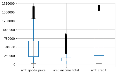
# other outliers
cols = ['amt_goods_price', 'amt_income_total', 'amt_credit']
for col in cols:
    df= df[np.abs(df[col]-df[col].mean()) <= (3*df[col].std())]
df.boxplot(column=['amt_goods_price', 'amt_income_total', 'amt_credit'])
Engineer a new feature, credit-to-income ratio. According to Investopedia, Lenders prefer to see a debt-to-income ratio smaller than 36%, with no more than 28% of that debt going towards servicing your mortgage.
# ratio
df['Credit_to_income'] = df['amt_credit'] / df['amt_goods_price']
df['Goods_to_credit'] = df['amt_goods_price'] / df['amt_credit']
Quantify the categorical (doing the dummies before looking at the correlation coefficient as I want categorical variables included)
df = pd.get_dummies(df)
Pearson correlation coefficient is the single fastest way to understand the relation between the dependent and independent variables. The correlation coefficients below are all very week, but among the strongest are ext_source_3, ext_source_2, ext_source_1, years_birth and years_employed.
In terms of the last two, the negative coefficient can be interpreted as the older the client gets and the more they work the same job, the less likely they are to default. Ext_source - normalized score from external data source, must be something like a credit score, have the strongest correlation with the target variable, the higher the ext_source, the less likely clients are to default.
# Find top correlations with the target
full_corr = df.corr()['target'].sort_values()
top10_corr = pd.concat([full_corr[:5],  full_corr[-6:]])
top10_corr
ext_source_3                           -0.178919
ext_source_2                           -0.160472
ext_source_1                           -0.155317
name_education_type_Higher education   -0.056593
code_gender_F                          -0.054704
days_last_phone_change                  0.055218
name_income_type_Working                0.057481
region_rating_client                    0.058899
region_rating_client_w_city             0.060893
days_birth                              0.078239
target                                  1.000000
Name: target, dtype: float64
MODEL TRAINING
# impute missing values
imp = Imputer(missing_values='NaN', strategy='mean', axis=0)
df_imputed = imp.fit_transform(df)
df = pd.DataFrame(df_imputed, columns=df.columns)
y = df.target
X = df[[col for col in df.columns if col !='target']]
Scaling might not improve the performance of logistic regression as the regression algorithm shrinks the coefficients of predictor variables with large ranges that do not effect the target variable.
scaler = StandardScaler()
Xs = scaler.fit_transform(X)
Xs = pd.DataFrame(Xs, columns=X.columns)
# Split into validation and training data
X_train, X_test, y_train, y_test = train_test_split(Xs, y, random_state=1)
Naive Baseline
Predicting the value of the majority class for all values give ROC AUC 0.5
df['y0.9'] = 0.9
print(roc_auc_score(y, df['y0.9']))
del df['y0.9']
0.5
Logistic Regression
Hyperparameters:
-
Regularization parameter C controls the amount of overfitting. The smaller C is, the stronger the regularization, so a lower value should decrease overfitting. Choosing the right C with gridsearch is strenuous on the system so instead I introduced regularization using L1 penalty (Lasso), which will also exclude several parameters by setting them to 0.
-
class_weightpenalizes mistakes in samples of class[i] with class_weight[i] instead of 1.class_weight="balanced"means replicating the smaller class until you have as many samples as in the larger one, but in an implicit way. -
solver: Specifying the solver to silence a deprecation warning. ‘liblinear’ solver is one that supports both L1 regularization.
# Specify the model
logreg = LogisticRegression(penalty='l1', class_weight='balanced', solver='liblinear')

# Fit it
model = logreg.fit(X_train, y_train)

# Score it
prob_y = model.predict_proba(X_test)
prob_y = [p[1] for p in prob_y]
print(roc_auc_score(y_test, prob_y))

# Predict class labels
y_pred=model.predict(X_test)
0.745791231303
Examining coefficients
# Get the models coefficients (and top 5 and bottom 5)
logReg_coeff = pd.DataFrame({'feature_name': X.columns, 'model_coefficient': model.coef_.transpose().flatten()})
logReg_coeff = logReg_coeff.sort_values('model_coefficient',ascending=False)
logReg_coeff['odds'] = np.exp(logReg_coeff['model_coefficient'])
logReg_coeff['P'] = logReg_coeff['odds'] / (1 + logReg_coeff['odds'])
logReg_coeff.head(5)
| feature_name | model_coefficient | odds | P | |
|---|---|---|---|---|
| 72 | obs_30_cnt_social_circle | 0.326753 | 1.386460 | 0.580969 |
| 3 | amt_credit | 0.228137 | 1.256258 | 0.556788 |
| 78 | flag_document_3 | 0.163409 | 1.177518 | 0.540762 |
| 35 | entrances_avg | 0.159622 | 1.173067 | 0.539821 |
| 65 | floorsmin_medi | 0.139569 | 1.149778 | 0.534836 |
logReg_coeff.tail(5)
| feature_name | model_coefficient | odds | P | |
|---|---|---|---|---|
| 30 | basementarea_avg | -0.193853 | 0.823779 | 0.451688 |
| 74 | obs_60_cnt_social_circle | -0.339017 | 0.712470 | 0.416048 |
| 5 | amt_goods_price | -0.357366 | 0.699516 | 0.411597 |
| 27 | ext_source_2 | -0.393003 | 0.675026 | 0.402995 |
| 28 | ext_source_3 | -0.458039 | 0.632523 | 0.387451 |
Interpretation:
-
Coefficients are the values for predicting the dependent variable from the independent variable. They are in log-odds units, corresponding to the likelihood that event will occur, relative to it not occurring. The highest coefficient here is ext_source_3, which, according to the columns descriptions, is a “Normalized score from external data source”, so it must be something akin to the credit score. Its coefficient says that for an increase of one unit ext_source_3, the odds of NOT defaulting (since the coefficient is negative) increase by 0.5.
-
It’s somewhat easier to interpret coefficients in odds, which we get by exponentiating the coefficient. The predictors with odds for above one are positively associated with default. The odds for
obs_30_cnt_social_circle, which is how many of client’s social surrounding hace defaulted 30 days past due, tell us that every additional friend who’d defaulted increase the odds of a credit applicant to default by 1.3 times, holding everything else constant. -
Lastly, the probability that someone who didn’t provide ‘document 3’ defaults is 54%.
We can asses the performance of the model by looking at the confusion matrix — a cross tabulation of the actual and the predicted class labels. Each row represents an actual class, while each column represents predicted class.
cnf_matrix = confusion_matrix(y_test, y_pred)
cnf_matrix
array([[47514, 21465],
       [ 2017,  4209]])
Confusion matrix can be confusing. Let’s do it the more explicit way. We see below that we correctly identified 4209 defaults, missed 2017 defaults and misclassified 21465 perfectly fine applications.
pd.crosstab(y_test, y_pred, rownames=['True'],
            colnames=['Predicted'], margins=True)
| Predicted | 0.0 | 1.0 | All |
|---|---|---|---|
| True | |||
| 0.0 | 47514 | 21465 | 68979 |
| 1.0 | 2017 | 4209 | 6226 |
| All | 49531 | 25674 | 75205 |
Another method to examine the performance of classification is the classification report.
- Precision: When it predicts yes, how often is it correct?
- Recall is the True Positive Rate: When it’s actually yes, how often does it predict yes?
- f1-score is a weighted average of the true positive rate (recall) and precision.
- Support is the number of samples of the true response that lies in that class.
print(classification_report(y_test, y_pred))
              precision    recall  f1-score   support

         0.0       0.96      0.69      0.80     68979
         1.0       0.16      0.68      0.26      6226

   micro avg       0.69      0.69      0.69     75205
   macro avg       0.56      0.68      0.53     75205
weighted avg       0.89      0.69      0.76     75205
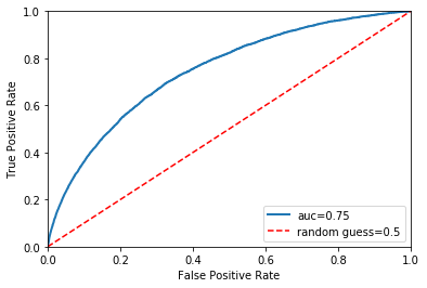
The ROC shows the True Positive Rate versus the False Positive Rate as a function of the threshold according to which we classify an instance as positive. To calculate a ROC AUC, we need to make predictions in terms of probabilities rather than a binary 0 or 1. The higher the score the better, with a random model scoring 0.5 and a perfect model scoring 1.0.
A single line on the graph indicates the curve for a single model, and movement along a line indicates changing the threshold used for classifying a positive instance. The prediction threshold should be set up based on HomeCredit risk tolerance, allowing it to compare performance across the entire probability spectrum.
y_proba = model.predict_proba(X_test)[::,1]
auc = roc_auc_score(y_test, y_proba)
fpr, tpr, thresholds = roc_curve(y_test, y_proba)
plt.plot(fpr, tpr, linewidth=2, label="auc="+str(round(auc, 2)))
plt.plot([0, 1], [0, 1], 'r--', label="random guess=0.5")
plt.axis([0, 1, 0, 1])
plt.xlabel('False Positive Rate')
plt.ylabel('True Positive Rate')
plt.legend(loc=4)
plt.show()
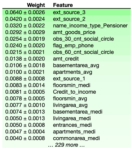
Permutation
Another way to understanding what features our model thinks are important is permutation importance, which answers the question: if we randomly re-order one of the features, leaving the rest as control features, how would that affect the accuracy of predictions? If accuracy drops considerably, the feature was important to the model. has a strong prediction power.
The first number in each row shows how much model performance decreased. The number after the ± measures how performance varied between multiple re-reshufflings. Negative values happen when random chance reshuffling caused the predictions on shuffled data to be more accurate.
Dan Becker included a microcourse on explainability in a Kaggle Learn module, here is where you can find more on permutaion: https://www.kaggle.com/dansbecker/permutation-importance
import eli5
from eli5.sklearn import PermutationImportance
perm = PermutationImportance(model, scoring = 'roc_auc', random_state=1).fit(X_test, y_test)
eli5.show_weights(perm, feature_names = X_test.columns.tolist())
Partial dependence plots
show how an individual feature affects the model’s prediction, marginalizing over other features. Due to the limits of human perception the size of the feature set is best limited to one or two of the most important ones. They can be interepreted similarly to the coefficients in regression models (but can capture more complex patterns). In the current sklearn version (20.3) PDP only works with a fitted gradient boosting model.
After a model is fit, we take a single observation and make a prediction for it, except we change one of the variables before making a prediction. Trying different values for that one variable, we trace how the target variable changes. We repeat the experiement with different variables and plot average predicted values on the vertical axis. Negative values mean target values would have been less than the actual average value for that predictor.
More info https://www.kaggle.com/dansbecker/partial-dependence-plots/
print(X.columns.get_loc("amt_goods_price"),
      X.columns.get_loc('ext_source_3'),
      X.columns.get_loc('years_birth'),
      X.columns.get_loc('years_employed'),
      X.columns.get_loc('amt_credit'))
5 28 244 245 3
from sklearn.ensemble.partial_dependence import partial_dependence, plot_partial_dependence
from sklearn.ensemble import GradientBoostingClassifier

gbc = GradientBoostingClassifier().fit(X, y)
my_plots = plot_partial_dependence(gbc, X=X, grid_resolution=5,
                                   # "feature_names" selects the variable names from df
                                   feature_names=X.columns,
                                   #"features" selects those variables from "feature_names" that we want to plot
                                   features=[244, 245])
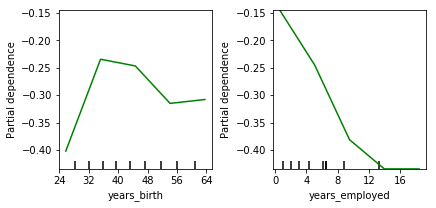
The plot on the left shows that the likelihood to default grows as people reach mid thirties, then falls till mid forties and slightly increases again. The likelihood to default is falling the longer you’re employed.
Partial Dependence Plot using the PDPBox library.
- The y axis is interpreted as change in the prediction from what it would be predicted at the baseline or leftmost value.
- A blue shaded area indicates level of confidence
from pdpbox import pdp
from pdpbox import get_dataset
from pdpbox import info_plots
# Create the data that we will plot
pdp_gtc = pdp.pdp_isolate(model=gbc, dataset=X,
                          model_features=X.columns,
                          feature='years_birth')
# plot it
pdp.pdp_plot(pdp_gtc, 'Age')
plt.show()
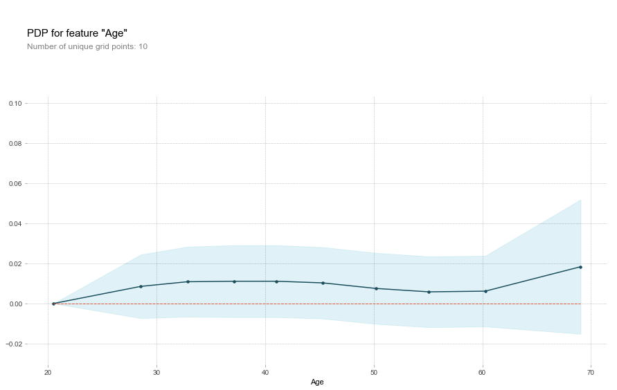
The global relationship between age and the probability of default is consistent with previous interpretations. The slight increase of default after sixties is a little more pronounced in this plot.
Conclusion
There are endless way predictive models including this one can be tinkered with to get more insights. I certainly could have looked closer at outliers, missing values, and come up with new features. But the point is that the future is algorithmic and work on machine learning interpretability is more important than ever. When building intelligence that supports us in our human goals, we must also constrain it by our human values. Interpretable models offer a safer, more productive, and ultimately more collaborative relationship between humans and intelligent machines.