This is a capstone project I created as part of graduating General Assembly’s Data Science Immersive program in New York in December 2017.
Bitcoin: bubble or blabber?
Background: Bitcoin has been in the news a lot recently. Its price has doubled four times this year and more people are now searching online for how to buy bitcoin than they are searching for how to buy gold. A situation where an asset’s price dramatically exceeds its intrinsic value points at a bubble, but what determines price and value? They aren’t scientific concepts, they are the co-creation of buyers and sellers whose needs and attitudes are constantly changing. A good proxy of people’s attitudes are social media and search engines. My project is looking at whether people’s attitude, as measured by Google Trend Score, can explain some of the bitcoin evaluation.
Question: Can we predict the value of bitcoins based on google searches? With what accuracy can change in price of Bitcoin be predicted using machine learning methods?
Data: Historical price on Bitcoin + Google Trend Score
Models: Time series, Support Vector Regression, Linear Regression, Naive Bayes (details in respective sections below)
Method:
-
Get data:
1.a. From Kaggle download the bitcoin data
1.b. From Google Trends download ‘interest’ score data
1.c. Merge the two on ‘Date’ -
EDA:
2.a. Trend graph
2.b. Heatmap
2.c. Correlation matrix -
Modelling:
3.a. Time Series
3.b. SVR
3.c. Linear Regression
3.d. Naive Bayes
Insights: Indeed some change in bitcoin’s value can be explained with change in search engine score, however the cryptomarket is volitile and susceptible to exogenous shocks, such as hitting evaluation milestones and/or comments from industry and government leaders.
Next steps:
- Rephrase the question into a binary classification problem and predict the direction of change.
- Set up a streaming API for Twitter to feed into models in real time.
- Determine whether ‘interest’ leads or trails the price of Bitcoin.
- Examine patterns of subsets of the price data, e.g. recent surges.
- Keep on tweaking the hyperparameters.
Libraries used:
import numpy as np
import pandas as pd
import seaborn as sns
import matplotlib.pyplot as plt
from datetime import datetime, timedelta

from sklearn.linear_model import LinearRegression
from sklearn.svm import SVR

%matplotlib inline
1. Get Data
1.b. bitcoin data
This dataset has the following features:
- Date : Date of observation
- btc_market_price : Average USD market price across major bitcoin exchanges.
- btc_total_bitcoins : The total number of bitcoins that have already been mined.
- btc_market_cap : The total USD value of bitcoin supply in circulation.
- btc_trade_volume : The total USD value of trading volume on major bitcoin exchanges.
- btc_blocks_size : The total size of all block headers and transactions.
- btc_avg_block_size : The average block size in MB.
- btc_n_orphaned_blocks : The total number of blocks mined but ultimately not attached to the main Bitcoin blockchain.
- btc_n_transactions_per_block : The average number of transactions per block.
- btc_median_confirmation_time : The median time for a transaction to be accepted into a mined block.
- btc_hash_rate : The estimated number of tera hashes per second the Bitcoin network is performing.
- btc_difficulty : A relative measure of how difficult it is to find a new block.
- btc_miners_revenue : Total value of coinbase block rewards and transaction fees paid to miners.
- btc_transaction_fees : The total value of all transaction fees paid to miners.
- btc_cost_per_transaction_percent : miners revenue as percentage of the transaction volume.
- btc_cost_per_transaction : miners revenue divided by the number of transactions.
- btc_n_unique_addresses : The total number of unique addresses used on the Bitcoin blockchain.
- btc_n_transactions : The number of daily confirmed Bitcoin transactions.
- btc_n_transactions_total : Total number of transactions.
- btc_n_transactions_excluding_popular : The total number of Bitcoin transactions, excluding the 100 most popular addresses.
- btc_n_transactions_excluding_chains_longer_than_100 : The total number of Bitcoin transactions per day excluding long transaction chains.
- btc_output_volume : The total value of all transaction outputs per day.
- btc_estimated_transaction_volume : The total estimated value of transactions on the Bitcoin blockchain.
- btc_estimated_transaction_volume_usd : The estimated transaction value in USD value.
b = pd.read_csv("datasets/bitcoin_dataset.csv", parse_dates=['Date'])
# df = pd.read_csv("datasets/bitcoin_dataset.csv")
# df.head()
b.shape
(2920, 24)
# b.info()
# b.sort_values('Date', axis=0, ascending=False)
# Make a boolean mask and re-assign to df
mask = (b['Date'] > '2012-11-07') & (b['Date'] <= '2017-11-07')
b = b.loc[mask]
b.shape
(1826, 24)
# get rid of 'btc_'
b = b.rename(columns={col: col.replace('btc_', '') for col in b.columns})
b.head()
| Date | market_price | total_bitcoins | market_cap | trade_volume | blocks_size | avg_block_size | n_orphaned_blocks | n_transactions_per_block | median_confirmation_time | ... | cost_per_transaction_percent | cost_per_transaction | n_unique_addresses | n_transactions | n_transactions_total | n_transactions_excluding_popular | n_transactions_excluding_chains_longer_than_100 | output_volume | estimated_transaction_volume | estimated_transaction_volume_usd | |
|---|---|---|---|---|---|---|---|---|---|---|---|---|---|---|---|---|---|---|---|---|---|
| 1094 | 2012-11-08 | 11.09790 | 10353750.0 | 1.149049e+08 | 358473.6925 | 3429.0 | 0.098442 | 0.0 | 182.0 | 11.133333 | ... | 3.671315 | 2.578037 | 30564.0 | 34985.0 | 8708635.0 | 12054.0 | 14375.0 | 1.465964e+06 | 221365.0 | 2456684.0 |
| 1095 | 2012-11-09 | 11.07000 | 10361000.0 | 1.146963e+08 | 211960.5342 | 3441.0 | 0.087469 | 0.0 | 202.0 | 12.800000 | ... | 3.851741 | 2.997240 | 28883.0 | 26851.0 | 8735486.0 | 11892.0 | 13836.0 | 9.956593e+05 | 188746.0 | 2089416.0 |
| 1096 | 2012-11-10 | 10.95899 | 10369000.0 | 1.136338e+08 | 168005.5734 | 3453.0 | 0.080664 | 0.0 | 277.0 | 9.883333 | ... | 6.891781 | 3.305210 | 24961.0 | 26595.0 | 8762081.0 | 9649.0 | 12441.0 | 4.819003e+05 | 116385.0 | 1275462.0 |
| 1097 | 2012-11-11 | 10.93900 | 10375600.0 | 1.134987e+08 | 187117.6000 | 3463.0 | 0.077176 | 0.0 | 264.0 | 15.833333 | ... | 9.348406 | 3.050546 | 21483.0 | 23728.0 | 8785809.0 | 8038.0 | 11160.0 | 3.757137e+05 | 70782.0 | 774286.0 |
| 1098 | 2012-11-12 | 11.18000 | 10382650.0 | 1.160780e+08 | 521129.2840 | 3474.0 | 0.080127 | 0.0 | 243.0 | 11.191667 | ... | 5.007497 | 3.205429 | 26835.0 | 24652.0 | 8810461.0 | 9925.0 | 12538.0 | 5.459378e+05 | 141148.0 | 1578039.0 |
5 rows × 24 columns
# b.describe()
# b.info()
# b.isnull().sum()
fig = plt.figure(figsize=(20,8))
ax = fig.add_subplot(111)
ax.plot(b['Date'], b['market_price'], lw=3)
ax.tick_params(labelsize=18)
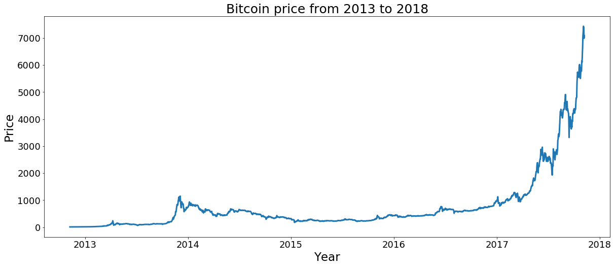
ax.set_title('Bitcoin price from 2013 to 2018', fontsize=25)
ax.set_ylabel('Price',fontsize=23)
ax.set_xlabel('Year',fontsize=23)
<matplotlib.text.Text at 0x1a142999e8>
# b.info()
1.b. Google data
‘Interest’ (over time, worldwide): Numbers represent search interest relative to the highest point on the chart for the given region and time. A value of 100 is the peak popularity for the term. A value of 50 means that the term is half as popular. Likewise a score of 0 means the term was less than 1% as popular as the peak.
g = pd.read_csv('datasets/google_bitcoin_2012.csv', header=1)
g.columns
Index(['Week', 'bitcoin: (Worldwide)'], dtype='object')
g.head()
| Week | bitcoin: (Worldwide) | |
|---|---|---|
| 0 | 2012-11-11 | 2 |
| 1 | 2012-11-18 | 1 |
| 2 | 2012-11-25 | 2 |
| 3 | 2012-12-02 | 2 |
| 4 | 2012-12-09 | 2 |
# g = g.rename(columns={'bitcoin: (Worldwide)':'Interest over time'}, inplace=True)
g = g.rename(columns={'Week': 'Date','bitcoin: (Worldwide)':'Interest'})
from datetime import datetime
g['Date'] = pd.to_datetime(g['Date'])
g.info()
<class 'pandas.core.frame.DataFrame'>
RangeIndex: 261 entries, 0 to 260
Data columns (total 2 columns):
Date        261 non-null datetime64[ns]
Interest    261 non-null int64
dtypes: datetime64[ns](1), int64(1)
memory usage: 4.2 KB
g.head()
| Date | Interest | |
|---|---|---|
| 0 | 2012-11-11 | 2 |
| 1 | 2012-11-18 | 1 |
| 2 | 2012-11-25 | 2 |
| 3 | 2012-12-02 | 2 |
| 4 | 2012-12-09 | 2 |
g.shape
(261, 2)
g.info()
<class 'pandas.core.frame.DataFrame'>
RangeIndex: 261 entries, 0 to 260
Data columns (total 2 columns):
Date        261 non-null datetime64[ns]
Interest    261 non-null int64
dtypes: datetime64[ns](1), int64(1)
memory usage: 4.2 KB
g.columns
Index(['Date', 'Interest'], dtype='object')
# g = g.set_index(g.iloc[0])
# g.set_index('Month')
# g = g.set_index(['Month'])

# g = g.set_index('Date') # inplace=True

# g.head()
fig = plt.figure(figsize=(15,6))
ax = fig.add_subplot(111)
ax.plot(g['Date'], g['Interest'], color='orange', lw=3)
ax.tick_params(labelsize=18)
ax.set_title('Bitcoin interest score from 2013 to 2018', fontsize=20)
ax.set_ylabel('Interest',fontsize=18)
ax.set_xlabel('Year',fontsize=18)
<matplotlib.text.Text at 0x1a1643efd0>
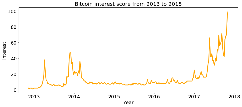
Interpretation:The graph above shows bitcoin’s search interest over the last 5 years. It currently strikes a value of 100, which translates into an all-time high. There was another spike around 2014 and a little before, but overall the interest over time has gone up. No obvious seasonality, but the [recent] trend is clear.
1.c. Join datasets
# dropping all dates that aren't in google df
df = pd.merge(b, g, how='inner', on=['Date'])

## other possibilities
# df = pd.merge(b, g, how="left", on=['Date'])
# df = pd.concat([b, g], axis=1)
df.shape
(261, 25)
df.isnull().sum().sum()
3
2. EDA
Data doesn’t have null values, so we can safely proceed discovering the relations within it.
2.a. Graph: Correlation between bitcoin search volume and its market price
# scale the Interest and the Price by dividing by the largest value of its own set
interest_scaled = df['Interest'] / 100
price_scaled = df['market_price'] / 1221.578347
date_ticks = df['Date']

# fig = plt.figure(figsize=(20,8))
# ax = fig.add_subplot(111)
fig, ax = plt.subplots(figsize=(15,6))
ax.plot(date_ticks[1:], price_scaled[1:], lw=3)#, figsize=(20,8))
ax.plot(date_ticks[1:], interest_scaled[1:], lw=3)#, figsize=(20,8))
plt.xlabel('Date', fontsize=20)
ax.tick_params(labelsize=18)
ax.set_title('Correlation between bitcoin interest and its price, 2013-2018', fontsize=20)
# plt.xlim(['2012-11-11', '2017-11-05'])
# ax.set_xlim([2013, 2018]) # Set the minimum and maximum of x-axis
plt.legend(['Price', 'Interest'], fontsize=15)
# plt.show()
<matplotlib.legend.Legend at 0x1a155f4978>
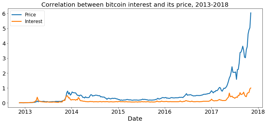
Interpretation: Visually we can already see that there is a correlation between the market price and interest. Let’s check if statistical algorithms confirm it.
fig, ax = plt.subplots(figsize=(15,6))
plt.scatter(df['Interest'], df['market_price'])
plt.xlabel('Interest', fontsize=15)
plt.ylabel('Price', fontsize=15)
# ax.tick_params(labelsize=18)
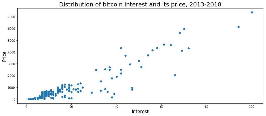
ax.set_title('Distribution of bitcoin interest and its price, 2013-2018', fontsize=20)
# plt.xlim(['2012-11-11', '2017-11-05'])
# ax.set_xlim([2013, 2018]) # Set the minimum and maximum of x-axis
# plt.legend(['Price', 'Interest'], fontsize=15)
# plt.show()
<matplotlib.text.Text at 0x1c1d1bf6d8>
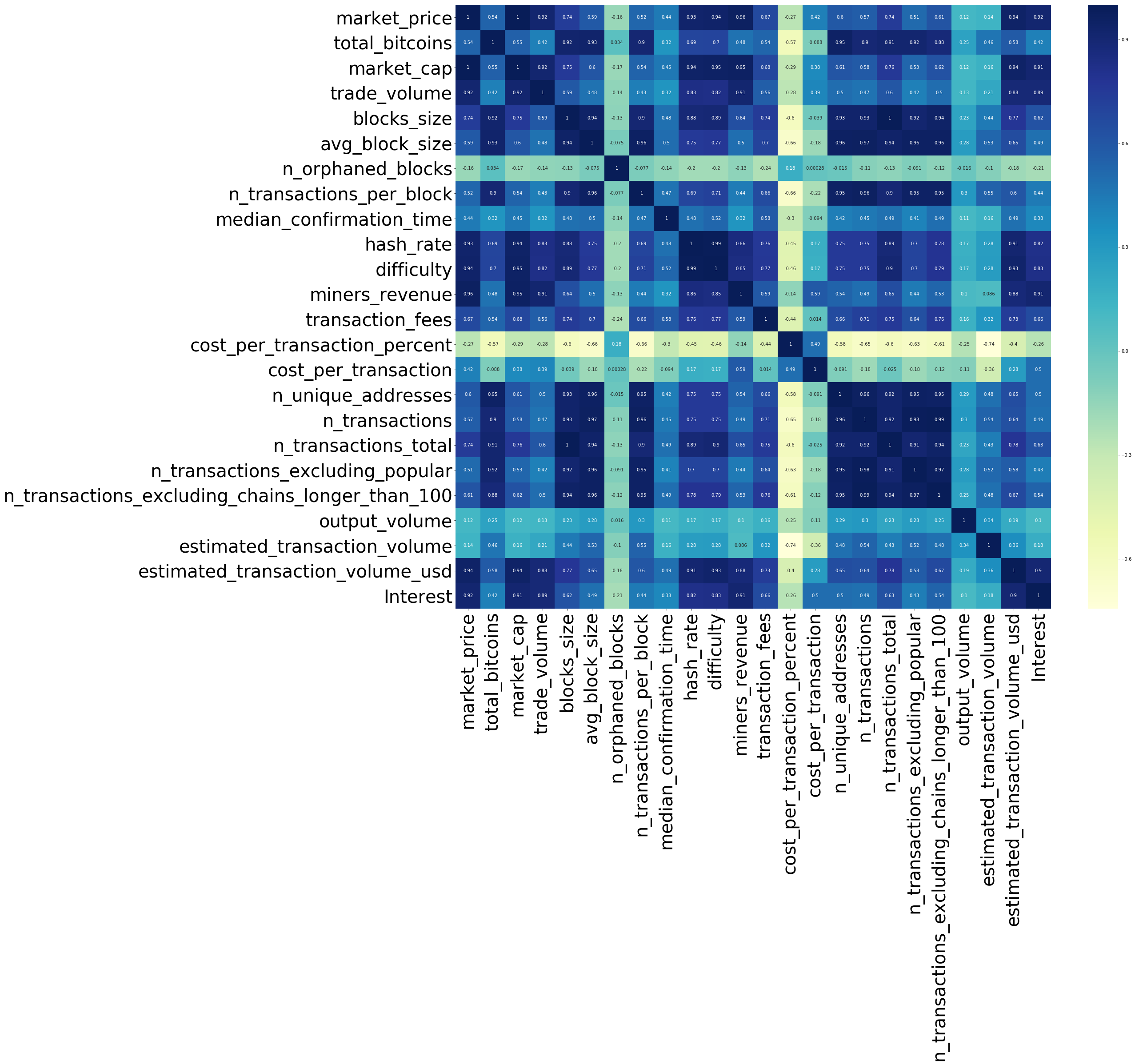
2.b. EDA: Heatmap of all features
corr = df.corr()
fig, ax = plt.subplots(figsize=(30, 25))
ax.tick_params(labelsize=40)
sns.heatmap(corr, annot=True, cmap='YlGnBu')
plt.show()
2.c. EDA: Correlation matrix
#get numerical features
numerics = ['int64', 'float64']
num_df = df.select_dtypes(include=numerics)
# Pearson correlation
corr = df.corr()['market_price']
# convert series to dataframe so it can be sorted
corr = pd.DataFrame(corr)
# label the correlation column
corr.columns = ["Correlation"]
# sort correlation
corr2 = corr.sort_values(by=['Correlation'], ascending=False)
corr2.head(15)
| Correlation | |
|---|---|
| market_price | 1.000000 |
| market_cap | 0.999003 |
| miners_revenue | 0.963504 |
| estimated_transaction_volume_usd | 0.941108 |
| difficulty | 0.937157 |
| hash_rate | 0.930085 |
| trade_volume | 0.917059 |
| Interest | 0.916211 |
| n_transactions_total | 0.744599 |
| blocks_size | 0.735276 |
| transaction_fees | 0.672164 |
| n_transactions_excluding_chains_longer_than_100 | 0.612018 |
| n_unique_addresses | 0.597402 |
| avg_block_size | 0.588632 |
| n_transactions | 0.568857 |
Interpretation: Bitcoin market price has a 91% correlation with our main feature, Interest.
3. MODELLING
3.a. Timeseries
Since data has a time dimension, I wanted to first use this one basic feature to see how much of the current surge in price is just a self-perpetuating moment. Formally, The question is then based JUST on a history of observations, what the next time unit’s price will be.
Time series is made up of Auto Regressive and Moving Average models, ARMA, that respectively capture the linear correlation between subsequent lags of time points and the error term of the model from previous time points, respectively.
y = df['market_price'].values.reshape(-1, 1)
X = df['Interest'].values.reshape(-1, 1)
from sklearn.model_selection import train_test_split, GridSearchCV
X_train, X_test, y_train, y_test = train_test_split(X, y, test_size=0.2)
print(X_train.shape, y_train.shape)
print(X_test.shape, y_test.shape)
(208, 1) (208, 1)
(53, 1) (53, 1)
from sklearn.preprocessing import StandardScaler
ss = StandardScaler()
Xs_train = ss.fit_transform(X_train)
Xs_test = ss.fit_transform(X_test)
/Users/Olga/anaconda3/lib/python3.6/site-packages/sklearn/utils/validation.py:475: DataConversionWarning: Data with input dtype int64 was converted to float64 by StandardScaler.
  warnings.warn(msg, DataConversionWarning)
Seasonal Decomposition
# seasonal_decompose() expects a DateTimeIndex on your DataFrame:
# df = df.set_index('Date')
# df.index.name = None
df['Date'] = pd.to_datetime(df['Date'])
# index=df['Date'].to_timestamp()
df['ts'] = df[['Date']].apply(lambda x: x[0].timestamp(), axis=1).astype(int)

## to reset index
# df.index.name = 'date'
# df.reset_index(inplace=True)
from statsmodels.tsa.seasonal import seasonal_decompose
result = seasonal_decompose(y, freq=20) # optional arg
result.plot();
type(result)
# You must specify a freq or x must be a pandas object with a timeseries index witha freq not set to None
statsmodels.tsa.seasonal.DecomposeResult
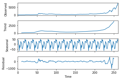
Interpretation:
- trend seems to accurately represent the observed values
- seasonality has clear regularity and fluctuations seems to be considerable, with -50 to 50
- residual doesn’t look stationary; does not follow seasonality
Dickey-Fuller test
To check if the data is stationary
# define Dickey-Fuller test
from statsmodels.tsa.stattools import adfuller
def test_stationarity(timeseries):

    #Determing rolling statistics
    rolmean = timeseries.rolling(window=12, center=False).mean()
    rolstd = timeseries.rolling(window=12, center=False).std()

    #Plot rolling statistics:
    fig = plt.figure(figsize=(12, 8))
    orig = plt.plot(timeseries, color='blue',label='Original')
    mean = plt.plot(rolmean, color='red', label='Rolling Mean')
    std = plt.plot(rolstd, color='black', label = 'Rolling Std')
    plt.legend(loc='best')
    plt.title('Rolling Mean & Standard Deviation')
    plt.show()

    #Perform Dickey-Fuller test:
    print('Results of Dickey-Fuller Test:')
    dftest = adfuller(timeseries, autolag='AIC')
    dfoutput = pd.Series(dftest[0:4], index=['Test Statistic','p-value','#Lags Used','Number of Observations Used'])
    for key,value in list(dftest[4].items()):
        dfoutput['Critical Value (%s)'%key] = value
    print(dfoutput)
# perform test
test_stationarity(df['market_price'])
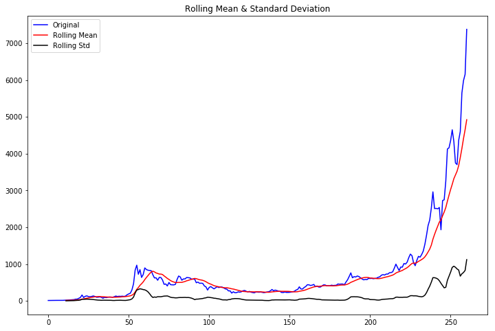
Results of Dickey-Fuller Test:
Test Statistic                   3.508900
p-value                          1.000000
#Lags Used                      13.000000
Number of Observations Used    247.000000
Critical Value (1%)             -3.457105
Critical Value (5%)             -2.873314
Critical Value (10%)            -2.573044
dtype: float64
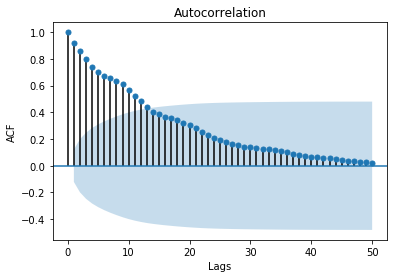
Autocorrelation of a series is the correlation between a time series and a lagged version of itself.
from statsmodels.tsa.stattools import acf
from statsmodels.graphics.tsaplots import plot_acf
print(acf(df.market_price, nlags=50))
plot_acf(df.market_price, lags=50);
plt.xlabel('Lags')
plt.ylabel('ACF')
[ 1.          0.91925934  0.85939797  0.79848796  0.73868008  0.70183552
  0.67154983  0.65448441  0.6377121   0.60961021  0.56711952  0.52439911
  0.484669    0.43783475  0.405981    0.38458242  0.36156547  0.35624696
  0.33914802  0.32155745  0.30252924  0.28399627  0.25318153  0.22838692
  0.20856838  0.18984676  0.17478248  0.16217524  0.15183748  0.1436451
  0.13716103  0.1305539   0.12544451  0.12285761  0.11872859  0.10990329
  0.09941787  0.08943473  0.08219397  0.07594753  0.06916554  0.06446443
  0.05899161  0.0555614   0.05039454  0.04285809  0.03723815  0.03343061
  0.02990163  0.02607458  0.02279817]


<matplotlib.text.Text at 0x1a160f2710>
# Partial autocorrelation (PACF) is similar to autocorrelation (ACF), but instead of just the correlation at increasing lags, it is the correlation at a given lag controlling for the effect of previous lags.
from statsmodels.tsa.stattools import pacf
from statsmodels.graphics.tsaplots import plot_pacf
# print(pacf(df.market_price, nlags=50))
plot_pacf(df.market_price, lags=50);
plt.xlabel('Lags')
plt.ylabel('PACF');
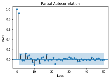
The data is not stationary, so we need to make it stationary to model.
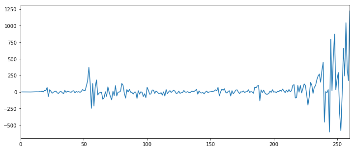
The most common way to make a timeseries stationary is to perform “differencing”- it removes trends in the timeseries and ensures that the mean across time is zero. In most cases there will only be a need for a single differencing, although sometimes a second difference (or even more) will be taken to remove trends.
# Difference the market price and plot.
df['market_price_diff']=df['market_price'].diff()
# data.head()
df['market_price_diff'].plot(figsize=(12, 5));

# Plot the ACF and PACF curves of the diff'd series
udiff= df['market_price_diff']
udiff.dropna(inplace=True)
plot_acf(udiff, lags=30);
plot_pacf(udiff, lags=30);
# Why diff? Warning! Don't diff blindly! Always check to see if you series is really stationary or not. You may need to diff more than once. How to know if your timeseries is stationary? You can formulate stationarity as a hypothesis and then test the hypothesis! An example of this approach is the Dickey-Fuller test
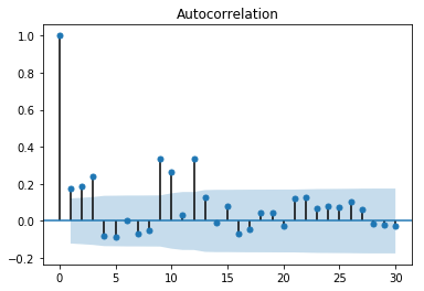
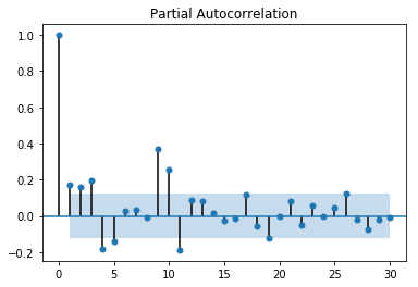
Interpretation: shaded region is the 95% confidence interval
Autoregression, or AR model is linear regression applied to timeseries - predicting timesteps based on previous timesteps. How many previous time steps should i use? only those significantly correlated
from statsmodels.tsa.arima_model import ARMA
ar1=ARMA(udiff.values, (1,0)).fit()
ar1.summary()
| Dep. Variable: | y | No. Observations: | 260 |
|---|---|---|---|
| Model: | ARMA(1, 0) | Log Likelihood | -1691.439 |
| Method: | css-mle | S.D. of innovations | 161.823 |
| Date: | Tue, 19 Dec 2017 | AIC | 3388.878 |
| Time: | 22:05:18 | BIC | 3399.560 |
| Sample: | 0 | HQIC | 3393.173 |
| coef | std err | z | P>|z| | [0.025 | 0.975] | |
|---|---|---|---|---|---|---|
| const | 29.5719 | 12.813 | 2.308 | 0.022 | 4.459 | 54.685 |
| ar.L1.y | 0.2170 | 0.068 | 3.195 | 0.002 | 0.084 | 0.350 |
| Real | Imaginary | Modulus | Frequency | |
|---|---|---|---|---|
| AR.1 | 4.6086 +0.0000j 4.6086 0.0000
Interpretation Lower value of AIC suggests “better” model, but it is a relative measure of model fit.
date_ticks.shape
(261,)
# # "In-sample" predictions
# # Get predictions from the time series:
date_ticks = df['Date']
fig, ax = plt.subplots(figsize=(12,5))
ax.plot(date_ticks[1:],
        udiff, lw=2, color='grey', ls='dashed')
ax.plot(date_ticks[1:], ar1.fittedvalues, lw=2, color='darkred')
plt.legend(['Actual values', 'In-sample predictions'], fontsize=15)
plt.show()
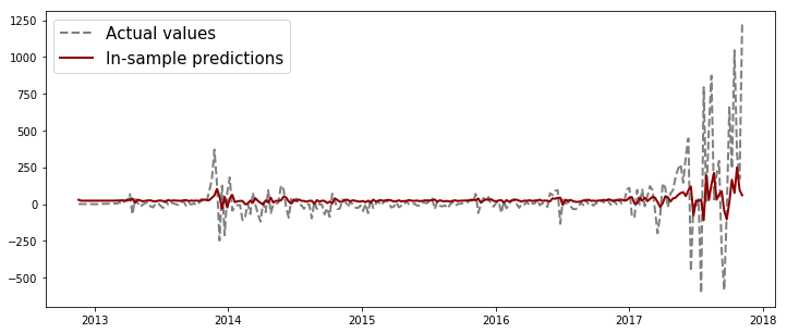
from sklearn.metrics import r2_score
print(r2_score(udiff, ar1.fittedvalues))
udiff.shape
type(ar1)
0.0379311476307


statsmodels.tsa.arima_model.ARMAResultsWrapper
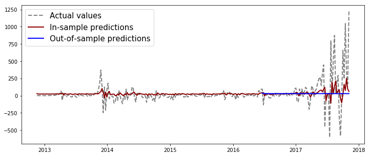
# # "Out-of-sample" predictions
# # What if we want to predict more than one time step into the future?
# # get what you need for predicting "steps" steps ahead
from statsmodels.tsa.arima_model import _arma_predict_out_of_sample
params = ar1.params
residuals = ar1.resid
p = ar1.k_ar
q = ar1.k_ma
k_exog = ar1.k_exog
k_trend = ar1.k_trend
steps = 73
oos_predictions = _arma_predict_out_of_sample(params, steps, residuals,
                               p, q, k_trend, k_exog,
                               endog=udiff.values, exog=None, start=100)
oos_predictions.shape
(73,)
date_ticks[101:].shape
(160,)
date_ticks[1:].shape
(260,)
fig, ax = plt.subplots(figsize=(12,5))
ax.plot(date_ticks[1:], udiff, lw=2, color='grey', ls='dashed')
ax.plot(date_ticks[1:], ar1.fittedvalues, lw=2, color='darkred')
ax.plot(date_ticks[188:],
        oos_predictions, lw=2, color='blue')
plt.legend(['Actual values', 'In-sample predictions', 'Out-of-sample predictions'], fontsize=15)
plt.show()
** Moving Average model**
(takes previous error terms as inputs. They predict the next value based on deviations from previous predictions. Prediciting on how wrong was i in predicting yesterdays values, it’s more of a compensating term.)
ma1=ARMA(udiff.values, (0, 1)).fit()
ma1.summary()
| Dep. Variable: | y | No. Observations: | 260 |
|---|---|---|---|
| Model: | ARMA(0, 1) | Log Likelihood | -1692.695 |
| Method: | css-mle | S.D. of innovations | 162.613 |
| Date: | Tue, 19 Dec 2017 | AIC | 3391.390 |
| Time: | 22:06:16 | BIC | 3402.072 |
| Sample: | 0 | HQIC | 3395.684 |
| coef | std err | z | P>|z| | [0.025 | 0.975] | |
|---|---|---|---|---|---|---|
| const | 29.0826 | 11.797 | 2.465 | 0.014 | 5.961 | 52.204 |
| ma.L1.y | 0.1701 | 0.063 | 2.680 | 0.008 | 0.046 | 0.295 |
| Real | Imaginary | Modulus | Frequency | |
|---|---|---|---|---|
| MA.1 | -5.8789 +0.0000j 5.8789 0.5000
fig, ax = plt.subplots(figsize=(12,5))
ax.plot(date_ticks[1:], udiff, lw=2, color='grey', ls='dashed')
ax.plot(date_ticks[1:], ma1.fittedvalues, lw=2, color='darkred')
plt.legend(['Actual values', 'Out-of-sample predictions'], fontsize=15)
plt.show()
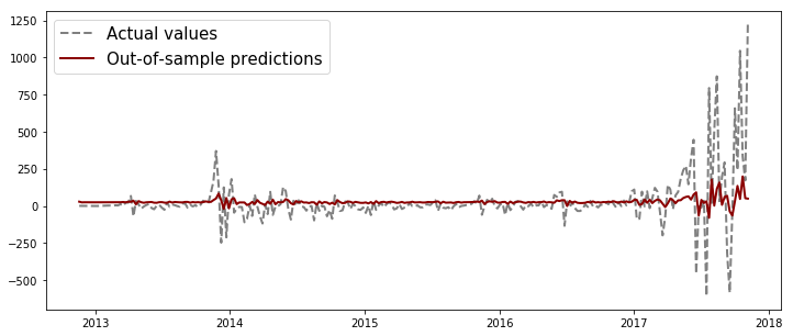
r2_score(udiff, ma1.fittedvalues)
0.028523326870250498
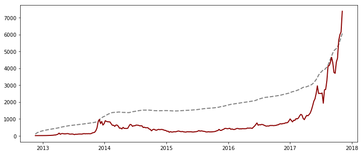
Full ARMA model
ar1ma1 = ARMA(udiff.values, (1,1)).fit()
ar1ma1.summary()
| Dep. Variable: | y | No. Observations: | 260 |
|---|---|---|---|
| Model: | ARMA(1, 1) | Log Likelihood | -1683.611 |
| Method: | css-mle | S.D. of innovations | 156.636 |
| Date: | Tue, 19 Dec 2017 | AIC | 3375.223 |
| Time: | 22:06:30 | BIC | 3389.465 |
| Sample: | 0 | HQIC | 3380.948 |
| coef | std err | z | P>|z| | [0.025 | 0.975] | |
|---|---|---|---|---|---|---|
| const | 92.2059 | 98.616 | 0.935 | 0.351 | -101.078 | 285.490 |
| ar.L1.y | 0.9917 | 0.011 | 93.838 | 0.000 | 0.971 | 1.012 |
| ma.L1.y | -0.8968 | 0.037 | -24.361 | 0.000 | -0.969 | -0.825 |
| Real | Imaginary | Modulus | Frequency | |
|---|---|---|---|---|
| AR.1 | 1.0084 +0.0000j 1.0084 0.0000||||
| MA.1 | 1.1151 +0.0000j 1.1151 0.0000
full_pred = df['market_price'].values[0]+np.cumsum(ar1ma1.fittedvalues)
fig, ax = plt.subplots(figsize=(12,5))
ax.plot(date_ticks[1:], full_pred, lw=2, color='grey', ls='dashed')
ax.plot(date_ticks[1:], df['market_price'][1:], lw=2, color='darkred')
plt.show()
3.b. Modelling: SVR
Time to use of my main feature, Google trend score, to answer the main question: Given there is a correlation between the interest and the bitcoin price, how accurately can change in the former predict change in the latter?
This is a regression problem, so after first trying out a Simple linear regression, I thought I’d try Support Vector Regression, since it’s better at picking up nonlinear trends in times series datasets.
A little about SVR: as a result of successful performance of SVM in real world classification problems, its principle of has been extended to regression problems too. Just like other regression techniques: you give it a set of input vectors and associated responses, and it fits a model to predict the response given a new input vector. Unlike other regression techniques, Kernel SVR, applies transformations to your dataset prior to the learning step. This is what allows it to pick up the nonlinear trend, unlike in linear regression.
from sklearn import svm, linear_model, datasets
from sklearn.model_selection import cross_val_score
# CREATE LAG PRICE
df['lag_price1'] = df['market_price'].shift(-1)
df['lag_price2'] = df['market_price'].shift(-2)
df['lag_price3'] = df['market_price'].shift(-3)
df['lag_price10'] = df['market_price'].shift(-10)
df = df.dropna(how = 'any')
# X = X.dropna(how = 'all')
# X = X.notnull()
# y = y.notnull()
y = df['market_price']#.values #.reshape(-1, 1)
# X = df[['Interest']]
X = df[['Interest', 'lag_price10', 'lag_price3', 'lag_price2', 'lag_price1']]
df.head()
| Date | market_price | total_bitcoins | market_cap | trade_volume | blocks_size | avg_block_size | n_orphaned_blocks | n_transactions_per_block | median_confirmation_time | ... | output_volume | estimated_transaction_volume | estimated_transaction_volume_usd | Interest | ts | market_price_diff | lag_price1 | lag_price2 | lag_price3 | lag_price10 | |
|---|---|---|---|---|---|---|---|---|---|---|---|---|---|---|---|---|---|---|---|---|---|
| 1 | 2012-11-18 | 11.83200 | 10425500.0 | 1.233545e+08 | 221950.3680 | 3563.0 | 0.094779 | 0.0 | 217.0 | 9.916667 | ... | 2.130380e+06 | 186303.0 | 2204342.0 | 1 | 1353214800 | 0.89300 | 12.60000 | 12.68000 | 13.53000 | 17.99999 |
| 2 | 2012-11-25 | 12.60000 | 10477050.0 | 1.320108e+08 | 338694.4484 | 3672.0 | 0.112150 | 0.0 | 219.0 | 13.216667 | ... | 8.956740e+05 | 110521.0 | 1392564.0 | 2 | 1353819600 | 0.76800 | 12.68000 | 13.53000 | 13.66548 | 20.68000 |
| 3 | 2012-12-02 | 12.68000 | 10515650.0 | 1.333384e+08 | 219481.9452 | 3773.0 | 0.065141 | 0.0 | 265.0 | 8.933333 | ... | 6.317366e+05 | 118130.0 | 1497889.0 | 2 | 1354424400 | 0.08000 | 13.53000 | 13.66548 | 13.48547 | 23.61458 |
| 4 | 2012-12-09 | 13.53000 | 10538475.0 | 1.425856e+08 | 413504.6784 | 3871.0 | 0.113781 | 0.0 | 398.0 | 13.083333 | ... | 8.741865e+05 | 117807.0 | 1593928.0 | 2 | 1355029200 | 0.85000 | 13.66548 | 13.48547 | 13.56998 | 25.60830 |
| 5 | 2012-12-16 | 13.66548 | 10560700.0 | 1.443170e+08 | 617988.9885 | 3987.0 | 0.134223 | 0.0 | 336.0 | 12.300000 | ... | 1.672238e+06 | 105974.0 | 1448181.0 | 1 | 1355634000 | 0.13548 | 13.48547 | 13.56998 | 13.52999 | 30.29777 |
5 rows × 31 columns
X.head()
| Interest | lag_price10 | lag_price3 | lag_price2 | lag_price1 | |
|---|---|---|---|---|---|
| 1 | 1 | 17.99999 | 13.53000 | 12.68000 | 12.60000 |
| 2 | 2 | 20.68000 | 13.66548 | 13.53000 | 12.68000 |
| 3 | 2 | 23.61458 | 13.48547 | 13.66548 | 13.53000 |
| 4 | 2 | 25.60830 | 13.56998 | 13.48547 | 13.66548 |
| 5 | 1 | 30.29777 | 13.52999 | 13.56998 | 13.48547 |
df.isnull().sum().sum()
0
from sklearn.model_selection import train_test_split
X_train, X_test, y_train, y_test = train_test_split(X, y, test_size=0.2)
print(X_train.shape, y_train.shape)
print(X_test.shape, y_test.shape)
(197, 5) (197,)
(50, 5) (50,)
from sklearn.preprocessing import StandardScaler
ss = StandardScaler()
Xs_train = ss.fit_transform(X_train)
Xs_test = ss.fit_transform(X_test)
print(Xs_train.shape)
print(Xs_test.shape)
(197, 5)
(50, 5)
np.mean(df['market_price'])
587.3596508246156
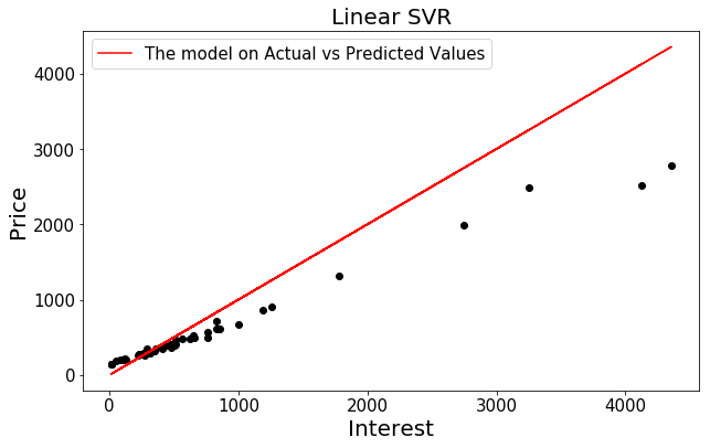
Linear SVR
svr_lin = SVR(kernel= 'linear', C= 1e3) # defining the support vector regression models
svr_lin.fit(Xs_train, y_train) # fitting the data points in the models
y_pred_lin = svr_lin.predict(Xs_test)
svr_lin.score(Xs_test, y_test) #Returns the coefficient of determination R^2 of the prediction
0.83667953307271892
# in linear SVM, the result is a hyperplane that separates the classes as best as possible.
# The weights represent this hyperplane, by giving the coordinates of a vector which is orthogonal to the hyperplane
svr_lin.coef_
array([[  12.47906365,    5.29824047,   20.2681008 ,  -27.8491547 ,
         590.61110206]])
fig, ax = plt.subplots(figsize=(10,6))
plt.scatter(y_test, y_pred_lin, c='k', label= 'Actual vs Predicted data')
# dots.set_label('dots')
plt.plot(y_test, y_test, color= 'red', label= 'Linear model')
# line.set_label('line')
plt.title('Linear SVR', fontsize=20)
plt.xlabel('Interest', fontsize=20)
plt.ylabel('Price', fontsize=20)
plt.tick_params(labelsize=15)
plt.legend(['The model on Actual vs Predicted Values'], fontsize=15)
plt.show()
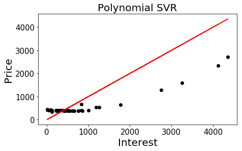
Polynomial SVR
svr_poly = SVR(kernel= 'poly', C= 1e3, degree= 2)
svr_poly.fit(Xs_train, y_train)
y_pred_poly = svr_poly.predict(Xs_test)
svr_poly.score(Xs_test, y_test)
0.64636842395965566
fig, ax = plt.subplots(figsize=(7,4))
plt.scatter(y_test, y_pred_poly, c='k')
plt.plot(y_test, y_test, color= 'red', label= 'Linear model')
plt.title('Polynomial SVR', fontsize=20)
plt.xlabel('Interest', fontsize=20)
plt.ylabel('Price', fontsize=20)
plt.tick_params(labelsize=15)
#plt.legend()
plt.show()
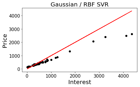
** Gaussian / RBF SVR**
svr_rbf = SVR(kernel= 'rbf', C= 1e3, gamma= 0.1)
svr_rbf.fit(Xs_train, y_train)
y_pred_rbf = svr_rbf.predict(Xs_test)
svr_rbf.score(Xs_test, y_test)
0.82504615525613534
fig, ax = plt.subplots(figsize=(7,4))
plt.scatter(y_test, y_pred_rbf, c='k')
plt.plot(y_test, y_test, color= 'red', label= 'Gaussian model')
plt.title('Gaussian / RBF SVR', fontsize=20)
plt.xlabel('Interest', fontsize=20)
plt.ylabel('Price', fontsize=20)
plt.tick_params(labelsize=15)
#plt.legend()
plt.show()
Interpretation:
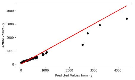
3.c. Modelling: Simple Linear Regression
** With three sets of features **
- All Features in df
- All the lagged versions of main predictor, price
- Just the main predictor, price
df = df.dropna(how='any')
y = df['market_price']#.values #.reshape(-1, 1)
# X = X = df[[col for col in df.columns if col !='market_price']].copy()
X = df[['Interest', 'lag_price10', 'lag_price3', 'lag_price2', 'lag_price1']]
# X = df[['Interest']]
from sklearn.model_selection import train_test_split, GridSearchCV
X_train, X_test, y_train, y_test = train_test_split(X, y, test_size=0.2)
print(X_train.shape, y_train.shape)
print(X_test.shape, y_test.shape)
(197, 5) (197,)
(50, 5) (50,)
from sklearn.preprocessing import StandardScaler
ss = StandardScaler()
Xs_train = ss.fit_transform(X_train)
Xs_test = ss.fit_transform(X_test)
from sklearn.linear_model import LinearRegression
lr = linear_model.LinearRegression()
lr.fit(Xs_train, y_train)
LinearRegression(copy_X=True, fit_intercept=True, n_jobs=1, normalize=False)
# how much of the variance in the response variable is explained by the model
lr.score(Xs_test, y_test)
0.92013363866339293
# check trained model y-intercept
print(lr.intercept_)
# check trained model coefficients
print(lr.coef_)
573.052267549
[  23.0055668    68.1836396   -65.93530847    5.72225034  605.62674702]
y_pred_lr = lr.predict(Xs_test)
y_pred_lr = lr.predict(Xs_test)
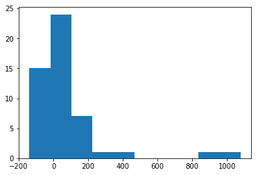
# Actual - prediction = residuals
residuals = y_test - y_pred_lr
np.mean(residuals)
70.67847338186604
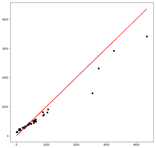
from sklearn.metrics import mean_squared_error, r2_score
rmse= np.sqrt(mean_squared_error(y_test, y_pred_lr))
r2 = r2_score(y_test, y_pred_lr)
print(rmse, r2)
233.303448443 0.920133638663
plt.figure(figsize=(7,4))
# plt.scatter(X, df['market_price'].values, c='k') #, s=30, c='r', marker='+') #, zorder=10)
plt.scatter(y_test, y_pred_lr, color='k')
plt.plot(y_test, y_test, color='r')
# plt.plot(y_pred_lr, '.')
# plt.plot(y_test, '-')
plt.xlabel("Predicted Values from - $\hat{y}$")
plt.ylabel("Actual Values - y")
# plt.plot([0, np.max(y_test)], [0, np.max(y_test)])
# plt.show()
<matplotlib.text.Text at 0x1c1d4ac128>
# plot residuals
fig = plt.figure(figsize=(10, 10))
ax = fig.gca()
ax.scatter(y_test, y_pred_lr, c='k')
ax.plot(y_test, y_test, color='r');
# iterate over predictions
# for _, row in df.iterrows():
#     plt.plot((row['X'], row['X']), (row['Y'], row['Linear_Yhat']), 'r-')
plt.hist(residuals)
(array([ 15.,  24.,   7.,   1.,   1.,   0.,   0.,   0.,   1.,   1.]),
 array([ -139.80928556,   -18.17008373,   103.4691181 ,   225.10831993,
          346.74752177,   468.3867236 ,   590.02592543,   711.66512726,
          833.3043291 ,   954.94353093,  1076.58273276]),
 <a list of 10 Patch objects>)
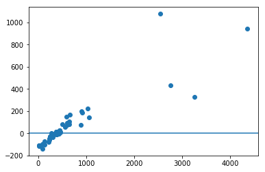
plt.scatter(y_test,residuals)
plt.axhline(0)
<matplotlib.lines.Line2D at 0x1c1c82f160>
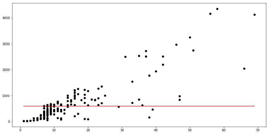
** 3.d. Modelling: Naive/Baseline prediction**
To see how the model can do with just the data it has
df['Mean_Yhat'] = df['market_price'].mean()
# Calculate MSE
df['Mean_Yhat_SE'] = np.square(df['market_price'] - df['Mean_Yhat'])
df['Mean_Yhat_SE'].mean()
463674.61500490666
fig= plt.figure(figsize=(15, 7.5))
ax= plt.gca()
ax.scatter(df['Interest'], df['market_price'], c='k')
ax.plot((df['Interest'].min(), df['Interest'].max()), (np.mean(df['market_price']), np.mean(df['market_price'])), color='r');
df['Mean_Yhat'] = df['market_price'].mean()
# Calculate MSE
df['Mean_Yhat_SE'] = np.square(df['market_price'] - df['Mean_Yhat'])
df['Mean_Yhat_SE'].mean()
463674.61500490666
# Find an optimal value for Elastic Net regression alpha using ElasticNetCV.
from sklearn.linear_model import Ridge, Lasso, ElasticNet, LinearRegression, RidgeCV, LassoCV, ElasticNetCV

l1_ratios = np.linspace(0.01, 1.0, 25)

optimal_enet = ElasticNetCV(l1_ratio=l1_ratios, n_alphas=100, cv=10,
                            verbose=1)
optimal_enet.fit(Xs_train, y_train)

print(optimal_enet.alpha_)
print(optimal_enet.l1_ratio_)
....................................................................................................................................................................................................................................................................................................................................................................................................................................................................................................................................................................................................................................................................................................................................................................................................................................................................................................................................................................................................................................................................................................................................................................................................................................................................................................................................................................................................................................................................................................................................................................................................................................................................................................................................................................................................................................................................................................................................................................................................................................................................................................................................................................................................................................................................................................................................................................................................................................................................................................................................................................................................................................................................................................................................................................................................................................................................................................................................................................................................................................................................................................................................................................................................................................................................................................................................................................................................................................................................................................................................................................................................................................................................................................................................................................................................................................................................................................................................................................................................................................................................................................................................................................................................................................................................................................................................................................................................................................................................................................................................................................................................................................................................................................................................................................................................................................................................................................................................................................................................................................................................................................................................................................................................................................................................................................................................................................................................................................................................................................................................................................................................................................................................................................................................................................................................................................................................................................................................................................................................................................................................................................................................................................................................................................................................................................................................................................................................................................................................................................................................................................................................................................................................................................................................................................................................................................................................................................................................................................................................................................................................................................................................................................................................................................................................................................................................................................................................................................................................................................................................................................................................................................................................................................................................................................................................................................................................................................................................................................................................................................................................................................................................................................................................................................................................................................................................................................................................................................................................................................................................................................................................................................................................................................................................................................................................................................................................................................................................................................................................................................................................................................................................................................................................................................................................................................................................................................................................................................................................................................................................................................................................................................................................................................................................................................................................................................................................................................................................................................................................................................................................................................................................................................................................................................................................................................................................................................................................................................................................................................................................................................................................................................................................................................................................................................................................................................................................................................................................................................................................................................................................................................................................................................................................................................................................................................................................................................................................................................................................................................................................................................................................................................................................................................................................................................................................................................................................................................................................................................................................................................................................................................................................................................................................................................................................................................................................................................................................................................................................................................................................................................................................................................................................................................................................................................................................................................................................................................................................................................................................................................................................................................................................................................................................................................................................................................................................................................................................................................................................................................................................................................................................................................................................................................................................................................................................................................................................................................................................................................................................................................................................................................................................................................................................................................................................................................................................................................................................................................................................................................................................................................................................................................................................................................................................................................................................................................................................................................................................................................................................................................................................................................................................................................................................................................................................................................................................................................................................................................................................................................................................................................................................................................................................................................................................................................................................................................................................................................................................................................................................................................................................................................................................................................................................................................................................................................................................................................................................................................................................................................................................................................................................................................................................................................................................................................................................................................................................................................................................................................................................................................................................................................................................................................................................................................................................................................................................................................................................................................................................................................................................................................................................................................................................................................................................................................................................................................................................................................................................................................................................................................................................................................................................................................................................................................................................................................................................................................................................................................................................................................................................................................................................................................................................................................................................................................................................................................................................................................................................................................................................................................................................................................................................................................................................................................................................................................................................................................................................................................................................................................................................................................................................................................................................................................................................................................................................................................................................................................................................................................................................................................................................................................................................................................................................................................................................................................................................................................................................................................................................................................................................................................................................................................................................................................................................................................................................................................................................................................................................................................................................................................................................................................................................................................................................................................................................................................................................................................................................................................................................................................................................................................................................................................................................................................................................................................................................................................................................................................................................................................................................................................................................................................................................................................................................................................................................................................................................................................................................................................................................................................................................................................................................................................................................................................................................................................................................................................................................................................................................................................................................................................................................................................................................................................................................................................................................................................................................................................................................................................................................................................................................................................................................................................................................................................................................................................................................................................................................................................................................................................................................................................................................................................................................................................................................................................................................................................................................................................................................................................................................................................................................................................................................................................................................................................................................................................................................................................................................................................................................................................................................................................

2.21673744488
1.0


....................................................................................................................................................................................................................................................................................................................................................................................................................................................................................................................................................................................................................................................................................................................................................................................................................................................................................................................................................................................................[Parallel(n_jobs=1)]: Done 250 out of 250 | elapsed:    4.9s finished
Evaluation
Is training error large?
Is training error « validation error?
# Cross-validate the ElasticNet $R^2$ with the optimal alpha and l1_ratio.
# How does it compare to the Ridge and Lasso regularized regressions?

enet = ElasticNet(alpha=optimal_enet.alpha_, l1_ratio=optimal_enet.l1_ratio_)

enet_scores = cross_val_score(enet, Xs_train, y_train, cv=10)

print(enet_scores)
print(np.mean(enet_scores))
[ 0.96272364  0.9809452   0.97588118  0.96270101  0.98324328  0.98899294
  0.9749028   0.79966757  0.98476662  0.98730991]
0.960113413788