Healthcare is integral to the quality of life in a modern society, yet the United States is the sickest of the rich countries: the costs in the US health-care system are higher than in any other capitalist countries, but this does not lead to better outcomes - 39 countries have longer life expectancies. (gapminder data)
This makes it a prime candidate for analytical intervention. In the last couple of years, Centers for Medicare and Medicaid Services (CMS) has been releasing some previously unaccessible data, including payments drug companies make to physicians (OpenPayments dataset), as well as doctors’ choices in Medicare’s prescription drug program (Medicare Part D dataset). ProPublica has previously analyzed the OpenPayments data in conjunction with the prescription data, showing that doctors who received money from drug and device makers — even just a meal – are two to three times as likely to prescribe brand-name drugs than doctors who didn’t. So I took the opportunity to get a closer look at what else drives the prescription choices (and what might be inflating drug prices and the opioid crisis).
The yearly data files consist of 2 datasets: the raw dataset assembled per a distinct combination of a doctor’s and drug’s name (about 25 million rows in 2017) and a summary table containing each doctors overall prescription costs and and claim counts for brand and generic drugs as well as demographic and health characteristics, such as patients’ insurance plans, incomes and disorders. Although it’s good practice to work with as unprocessed data as possible, I was more interested in the overall demographic and utilization so I chose to work with the aggregated dataset.
After wrangling the data from 2015 to 2017 into my own dataset using a DB Browser for SQLite, here are the spending and volume highlights I found:
- Medicare could have saved $85 billion on average per year if a generic drug was prescribed every time in plave of a brand. This number is consistent with (offical reports).
- Brand drugs cost 80% of total spending on drugs, on average per year, while brand drug claims are only 18% out of total drug claims.
- Amount of prescribing doctors rose by almost 3% on average
- Total amount of brand prescription has fallen by almost 4% and total amount of generic has risen by 3% on average
- Total spending has increased 8% on average (while average annual inflation rate is 3.2%)
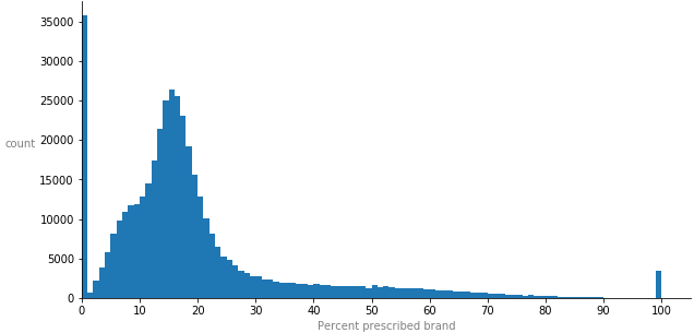
To have an estimator variable of each doctor’s prescription habits, I’ve calculated the percentage of brand-name drugs each doctor prescribed out of total - as the dependent variable. The majority of doctors prescribed close to 0 brand drugs, average doctor prescribed 18% brand, and there are 3,500 doctors who only prescribed brand drugs. This is what the distribution of percent prescribed brand looks like:
To further compare doctors without being misled by the size of their practices, I engineered proportional representations (cost per claim, cost per beneficiary and claim per beneficiary) for each characteristic of their practice.
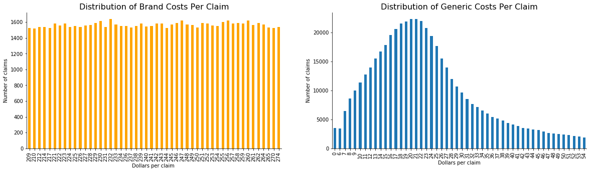
This is how brand and generic costs per claim are distributed: for each brand drug cost there are the same amount of claims, but generic costs follow a more normal (still slightly skewed) distribution with diffirent amounts of claims for each cost amount.
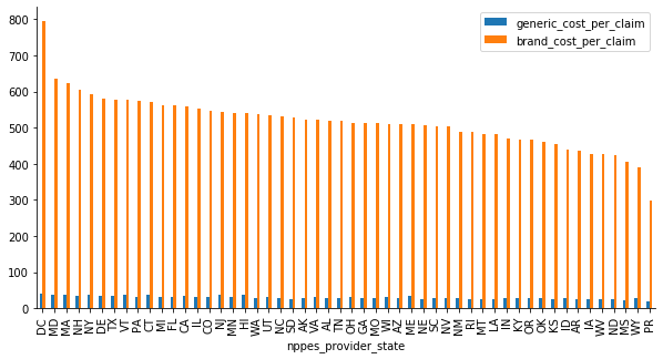
Across the country, brand cost per claim are on average 17 higher than generic cost per claim:
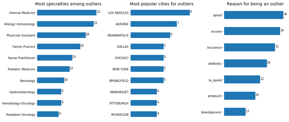
Looking at the boxplot distributions of all the different characteristics of doctors’ practices (which will be too bulky to include in this writeup), most values cluster around 0 and you mostly see a long tail of outliers - doctors whose claims and costs are way higher than the majority of the doctors’. So I decided to collect those into one group and look closer into them. Here’s what they practice, where they live and, what characteristic they are an outlier for:
To see how my features are correlated with how much brand drugs an outlier doctor prescribes, we can calculate a Pearson’s correlation coefficient, the most common measure of relationship between two variables. 6 out of top 10 most correlated features were the ones I engineered, but here are the top 3:
-
nonlis_cost_per_claim (0.576560): The higher the cost per claim for beneficiaries without a low-income subsidy charged, the more brand drugs a doctor prescribes. -
pdp_cost_per_claim (0.484523): The higher the cost per claim beneficiaries covered by standalone PDP are charged, the more brand drugs a doctor prescribes. -
La_opioid_prescriber_rate (-0.454956): The higher the percent of long-acting opioid claims expressed in terms of total opioid claims, the less brand drugs a doctor prescribes.
To look further into the interactions between variables and their relative levels of importance, let’s see how a single tree (good resolution):
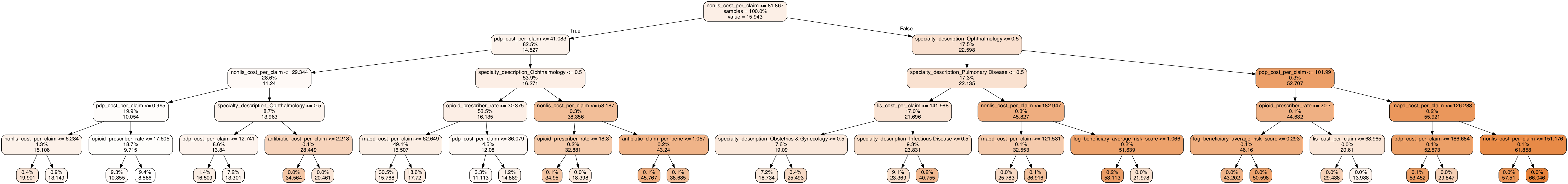
Starting at the root node (depth 0, at the top): the tree decides that the single best question it can ask to separate the doctors’ practices into two groups is whether their cost per claim for beneficiaries without a low-income subsidy is less or more than 82 dollars. Then we ask a different follow-up question, recursively splitting data into many different areas, assigning a single value to every point that lands in a certain area. The final endpoints in a tree are known as leaves. Every point placed in a certain leaf is given the same value, the average of the known points in that leaf. To find out doctors who prescribe the highest percent of brand, we follow the branches down to the brightest orange leaf. Out of 5 questions (the amount controlled by hyperparameter “max_depth”) our tree asks 1 question related to doctor’s specialty and 4 related to patient’s income and type of plan.
One limitation of trees is the natural blockiness of their predictions. It is rare for natural events to share in this blocky nature, so generally trees make relatively inaccurate predictions on data.
I also fit the data to Linear Regression, Random Forest and Ensemble’s Voting Regressor models. The latter slightly underperformed compared to Random Forest, which tells me the component models are not perfectly independent. When re-training on the top 20 features, performance did not change, which tells me the model is not biased. When I used only the engineered features, I got the best performance yet. Looking at the residual plots, however, all other models’ and feature subsets had random distributions of fitted VS residual values, while engineered features had some quite clear patterns.
The features that Random Forest deemed important agree with what we’ve already seen: costs and counts for patients’ types of income and plans. It seems like the general theme among doctors overprescribing brand-name drugs is who picks up the bill.
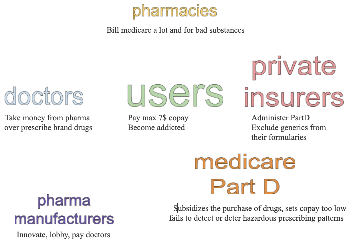
As an analyst, I’m not supposed to point the decision-makers in any particular direction, but rather to expand the perspective of available options to choose from. However, it seems from this research that while PartD’s very structure promotes cost growth, drug manufacturers and health insurers will be the ones benefitting from it, at the expense of patients and taxpayers.